In Graphics Programming, we refer to Geometry Processing as the set of all the necessary operations needed to transform 3D vertices into 2D coordinates on the screen. This part of the graphics pipeline in particular is full of 3D math and complex coordinate transformations, and therefore it’s easy to lose your train of thoughts somewhere down the road. In this post i want to share my understanding of the subject, and my personal implementation in OpenGL.
Transformations
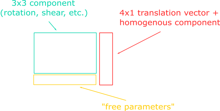
First of all, let’s deal with the elephant in the room. What is a transformation? You can think about it in a math fashion, or in a computer science fashion. Starting with the first interpretation, a transformation is a matrix that, when applied to an input vector, warps it from its input space to an output space. The net effects of a transformation can be one or more between the following: translation, rotation, scaling, reflection, shearing, stretching and squeezing. While a translation can be expressed with a simple 3D vector, all the other fancy effects can be described with a 3×3 matrix. If we bundle up these two components in the same matrix we get an affine transformation, which is characterized by its ability of preserving collinearity (hence transforming parallel lines into other parallel lines). An affine transformation can be represented by a 4×4 matrix containing a 3×3 component in the upper left corner and a translation component in the fourth column. If we pack the information in this way, we need to use 4D input vectors in order for our transformations to apply the translation effect as well. Working with 4D vectors moves us away from the Euclidean space into the domain of homogenous coordinates. The final step to complete our transformation matrix is to add a 3D vector in the fourth row, usually set equal to Vec3(0, 0, 0). These three numbers are effectively “free parameters” because we can design them in order to suit our needs. We will see one neat trick that’s possibile to achieve thanks to them in a little bit, when we’ll talk about the perspective projection.
Homogenous coordinates have very interesting properties. With them it’s possible to express the location of a point in 3D space by dividing the x, y and z components of the 4D homogenous vector by w. This operation hints that the 3D Euclidean space is actually a subset of the 4D homogenous space obtained by setting w = 1. Under this condition, a line in 4D is projected to a point in 3D and this is also why these coordinates are called “homogenous”: scaling a 4D vector by any amount (greater than zero) still produces the same projected point in 3D space, after dividing by the w-component. A necessary consequence of these properties is that, when the homogenous coordinate is equal to one, the geometrical interpretation of the 4D vector is equal to a point in Euclidean space. When w = 0, however, it’s not possible to find anymore an intersection between the 4D line and any point in 3D space. We talk about “point at infinity” or “direction”, to differentiate with respect to the previous case. So, points have a w = 1 and directions have a w = 0, and the usual math rules apply exactly like in the case of two 4D vectors. Directions can be summed, producing another direction (head-to-tail method), or a point and a direction can be summed in order to produce a translated point. The difference between two points, instead, produces a direction since the w-components subtract to zero. Finally, the sum of two points produces another point with coordinates equal to the averaged components (remember that we need to divide by w!). A very good discussion about points and directions can be consulted in this presentation https://www.youtube.com/watch?v=o1n02xKP138. As a final note about the mathematical interpretation of transformations, it’s important to keep in mind that matrix multiplication is not commutative, and that the correct composition of multiple consecutive transforms is obtained by applying them in a right-to-left fashion.
According to the computer science interpretation instead, a transformation is just a data structure, usually a 4×4 multidimensional array of floating point values. The data storage in the multidimensional array can be executed by placing row values as contiguous in memory (row-major order) or column values instead (column-major order). I personally prefer the latter, since column vectors are generally more useful in computer graphics, and the acces to a column vector in a column-major ordered matrix is fast and simple in C++. However, their disadvantage is that in the visual studio debugger all matrices appear as transposed! This can be solved by building custom debug services, such as visualization tools and introspections, or by applying a further transposition to counteract the previous one.
The Model-View-Projection (MVP) Matrix
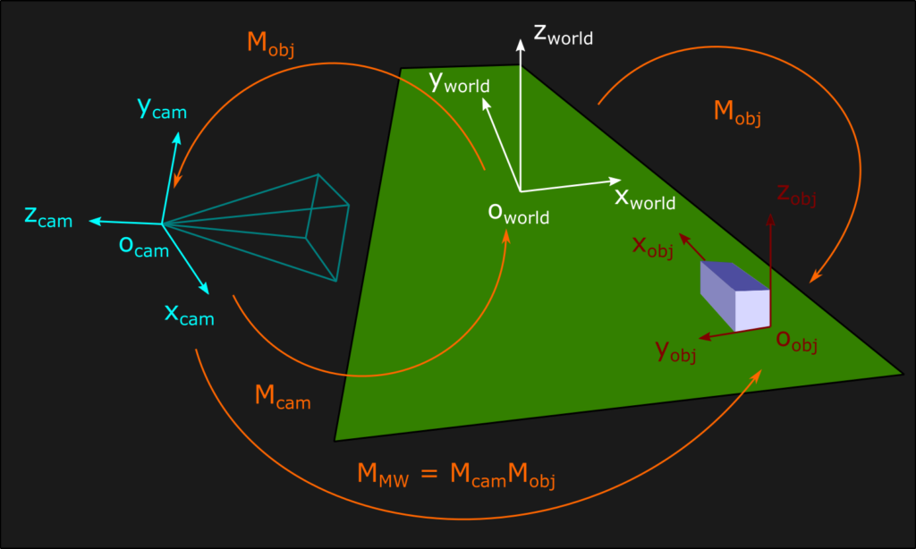
Now let’s talk about why transformations are important in computer graphics. All the graphic assets of a videogame, from images to 3D models, exist inside their own coordinate system called object space. Inside the virtual environment simulated by a videogame, instead, the vertices of all 3D models exist into a coordinate system that is often called world space (or global space). The world space acts as a big container, is unique and expresses the position and the orientation of every object with respect to its origin. The transformation that moves each vertex from its object space to the global world space is called object transform (or model transform), in short Mobj. The game logic usually dictates how to move each object, and therefore our application is responsible for defining all the object transforms. However, there is one object transform in particular that needs some special attention: the camera. Just like all other objects, the camera has its position and orientation expressed in world space, but sooner or later every graphics simulation needs to see the rest of the world through its eyes. For this to happen, it’s necessary to apply to each object in world space the inverse of the object transform relative to the camera. After this transformation vertices exist inside the camera space, a right-handed coordinate system centered on the world origin that may have the positive y direction going upward, and the positive z going in the opposite direction of the camera gazing (this is the convention used in my engine). Alternatively, the y can be top-down and the positive z can be directed as the camera gazing, if we want to keep the coordinate system as right-handed. Since the camera is special, and also because it’s easy to be confused by all this nomenclature and mathematical reasoning, we usually define a camera transform (or view transform) Mcam to differentiate it from all other object transforms. In the graphics programming literature, however, the camera transform is defined according to at least two different conventions. Technically, the transform that moves the camera from the origin of the world to its desired position is an object transform, but often this is the one defined as camera transform. In this case, by applying the inverse of the camera transform we are able to work inside the camera space. Other sources instead consider the forward transform as an object transform, and define the inverse transform as the actual camera transform. This last interpretation is my personal favourite and this is the convention i follow in my engine. Now, having formalized our approach, let’s discuss some practical implementation. Computing the inverse of a matrix is usually an expensive operation, but sometimes math comes in our aid! In the case of orthogonal matrices like rotations, the inverse is equal to the transpose (i’ll save you the proof, you can find it literally everywhere all over the internet). For homogenous transformations, the inverse computation takes the following form (also easy to demonstrate):
When i deal with a matrix transformation i usually like to store both forward and inverse transforms inside a struct. This allows to pre-compute both of them, saving me an unnecessary runtime burden. For example, the camera transform can be computed as follows:
// Transform4f is derived from a more generic Matrix4f, a column-major multidimensional array
// in which we keep the fourth row equal to [0, 0, 0, 1]. All the needed math functions and
// operator overloadings are omitted for the sake of brevity. Let's see only how to compute
// the inverse of an orthogonal transform
Transform4f Transform4f::InvOrtho(const Transform4f& T)
{
Transform4f result = Transform4f::Transpose(T);
result.setTranslation(-(result * T.getTranslation()));
return result
}
struct transform4f_bijection{Transform4f forward;Transform4f inverse;};// Define the object tansform for the camera. In this case the constructor takes a// 3x1 translation vector and a 3x3 rotation matrix representing camera position
// and orientationTransform4f camObjectTransform(rotationMatrix, translationVector);// We define the camera transform as the inverse object transform for the cameratransform4f_bijection cameraTransform;cameraTransform.forward = Transform4f::InvOrtho(camObjectTransform);cameraTransform.inverse = camObjectTransform;
As a final note on camera transforms, consider that it’s possible to compose them with the object transforms in order to create the model-view transform, which allows to move objects directly inside the camera space without passing through the world space. In order to have an intuitive graphical understanding of the whole situation, we can use by convention an arrow that points from the source space to the destination space, indicating the flow of all the various transforms:
After applying the model-view transform we are in camera space and we are ready for the next step: the projective transform, which brings us inside the clip space. As you may know by simply playing any videogame ever, during the simulation we are only able to see what the camera allows us to see. Every geometry that is not visible by the camera needs to be clipped because it would be a waste of resources to be rendered otherwise. The projection allows us to determine which vertex has to be rendered, and it achieves this goal by mapping the view volume into the clip space. The view volume is simply a collection of clip planes: top (t), bottom (b), left (l), right (r), near (n) and far (f). As far as the clip space is concerned, instead, it usually has the x and y directions mapped in the [-1, 1] range, and it may have the z direction mapped just like the other ones (OpenGL) or inside the [0, 1] range (Direct3D, Vulkan, Metal, consoles). While the mapped ranges are the same for different types of projection, the view volumes changes substantially instead. For orthographic projections the view volume is a cube, while for perspective projections it has the shape of a frustum:
![]()
Orthographic projection
After the orthographic transform all parallel lines in world space are going to be projected as parallel lines in the projection plane (xp=xcam, yp=ycam), so an affine transform will be just fine. The orthographic matrix needs to map the x and y dimensions of the projection plane in the range [-1, 1]. In order to achieve that, let’s apply the matrix multiplication rule to the first element of the 4D input vector. If we use two variables A and B as parameters of the transformation, we can determine their values by applying the left and right planes constraints. The same reasoning can be applied also to the y-component for symmetry:
 x_{clip} = A*x_{cam} + B

 \begin{cases} 1 & = & A*r + B \\ -1 & = & A*l + B \end{cases}   \hspace{45pt} \Rightarrow \hspace{18pt} \begin{cases} A & = & (1 - B) / r \\ -1 & = & (1 - B) * l/r  + B \end{cases}

 \begin{cases} A & = & (1 - B) / r \\ -r & = & l - B*l + B*r \end{cases}   \hspace{17pt} \Rightarrow \hspace{18pt} \begin{cases} A & = & 2 / (r - l) \\ B & = & - (r + l) / (r - l) \end{cases}

 y_{clip} = A*y_{cam} + B

 \begin{cases} A & = & 2 / (t - b) \\ B & = & - (t + b) / (t - b) \end{cases}
For the depth range instead we are going to consider a mapping inside the [0, 1] interval, even if we are working in OpenGL. This is more in line with all the other graphics API and it improves the depth buffer precision as well. We can define two variables A and B in position (3, 3) and (3, 4) of the orthographic matrix in order to specify the mapping for near and far planes. Applying the same reasoning as before, we can write the following expressions:
 z_{clip} = A*z_{cam} + B

 \begin{cases} 0 & = & -A*n + B \\ 1 & = & -A*f + B \end{cases}   \hspace{35pt} \Rightarrow \hspace{23pt} \begin{cases} A & = & B/n \\ 1 & = & -B * f/n  + B \end{cases}

 \begin{cases} A & = & B/n \\ n & = & -B*f + B*n \end{cases}   \hspace{17pt} \Rightarrow \hspace{23pt} \begin{cases} A & = & 1 / (n - f) \\ B & = & n / (n - f) \end{cases}
Finally, let’s see an implementation in C++ that also pre-computes and stores the inverse transformations. Note how when the viewing volume is symmetrical along the x and y directions, both the non-diagonal contributions are nullified (r+l and t+b compensate themselves). Only the asymmetrical depth range generates a non-diagonal element:
// We use a more generic Matrix4f struct, instead of the previous Transform4f, in order// to create a common ground with the perspective projection (see the next section). The// perspective, infact, needs to use also the free parameters of the transformmatrix4f_bijection orthographicTransform(float width, float height, float n, float f){matrix4f_bijection result;float w = 2.0f / width;float h = 2.0f / height;float A = 1.0f / (n - f);float B = n / (n - f);result.forward = Matrix4f( w , 0.0f, 0.0f, 0.0f,0.0f, h , 0.0f, 0.0f,0.0f, 0.0f, A , B ,0.0f, 0.0f, 0.0f, 1.0f);result.inverse = Matrix4f(1.0f/w, 0.0f, 0.0f, 0.0f,0.0f, 1.0f/h, 0.0f, 0.0f,0.0f, 0.0f, 1.0f/A, -B/A,0.0f, 0.0f, 0.0f, 1.0f );// Place a breakpoint here and check the correct mapping#if _DEBUG_MODEVector4f test0 = result.forward * Vector4f(0.0f, 0.0f, -n, 0.0f);Vector4f test1 = result.forward * Vector4f(0.0f, 0.0f, -f, 0.0f);#endifreturn result;}
Perspective projection
The perspective transform is a different beast compared to the orthographic one. In this projection, the x and y-components are scaled with the inverse of the z-component, in order to represent our visual perception of distant objects being smaller than close ones. This is inherently a non-linear operation and therefore the affine transforms are no longer sufficient to describe our problem. Mathematically, we can justify this truth by observing that affine transformations cannot possibly apply a division for one of their input values, which is what we would need to do with the z-component. Intuitively, instead, we can just consider that affine transformations are invariant with respect to parallel lines, but the perspective is not! Think about train tracks disappearing into the horizon: they are clearly parallel, or at least we hope so for the trains and all the passengers, but visually they seem to converge up to some point at infinity. This problem can be solved by homogenous coordinates and the “free parameters” of the projection matrix we mentioned before. Homogenous coordinates perfectly suit our needs because they actually apply a division by one of their input values, the w-component. Considering that all modern graphics API perform automatically the perspective divide as a GPU operation, we just need to use one of our free parameters in order to place -z (remember our coordinate system convention) into the w-component. This can be achieved by setting the (4, 3) component of the perspective transform to -1, and then the matrix multiplication rule is going to apply its magic.
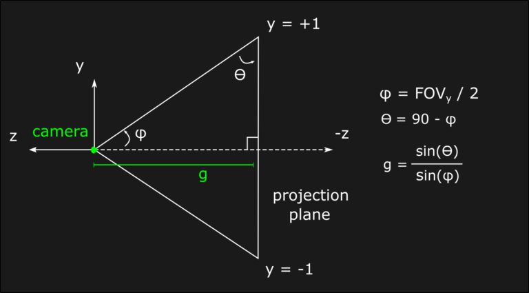
Another consequence of the perspective transform is that the postion of the projection plane, or in other words the focal length, is now very relevant to the visual outcome because of the inverse depth scaling. In fact, by moving the projection plane closer to the scene it’s possible to see a zoom effect. In order to understand the mathematical relation between depth, focal length and projection planes is sufficient to apply the similar triangles formula. In this model, the common vertex is the camera while the bases are projection plane and an arbitrary depth value into the game world:
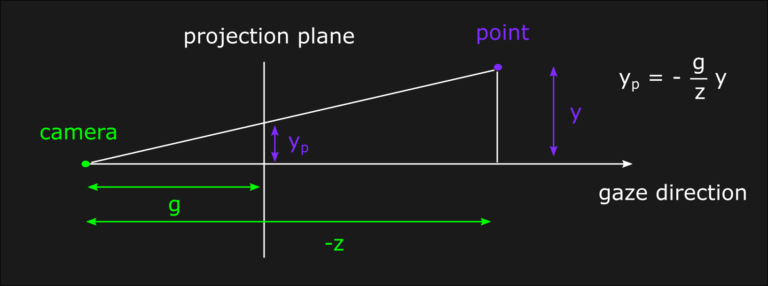
The same reasoning can be applied also for the x-component, which is the one orthogonal to the screen in the previous figure. This information, together with our desired clip values, allows us to design the perspective transform using a similar approach to the one we used in the orthographic case. We determine the value of A and B after applying the matrix multiplication, only that this time B is in a different position ([1, 3] for x and [2, 3] for y in a column-major case) and we also need to consider the perspective divide:
 x_{clip} = A*x_{p} + B*z_{p}

 \begin{cases} 1 & = & A*r + B*z_{p} \\ -1 & = & A*l + B*z_{p} \end{cases}   \hspace{25pt} \Rightarrow \hspace{25pt} \begin{cases} B & = & (1 - A*r) / z_{p} \\ -1 & = & A*l + 1 - A*r \end{cases}

 \begin{cases} B & = & (1 - A*r) / z_{p} \\ A & = & 2 / (r - l) \end{cases}   \hspace{29pt} \Rightarrow \hspace{26pt} \begin{cases} B & = & -(r + l) / (z_{p}*(r - l)) \\ A & = & 2 / (r - l) \end{cases}

Substitute the perspective equations inside the transform:

 \begin {cases} x_{p} & = & g * x_{cam}/z_{cam} \\ z_{p} & = & z_{cam} \end{cases} \hspace{13pt} \Rightarrow \hspace{8pt}   x_{clip} = \frac{2*g*x_{cam}}{-z_{cam} * (r - l)} + \frac{z_{cam} * (r + l)}{-z_{cam} * (r - l)}

Since the perspective divide will happen after the transform,
the desired A and B values are the following:

 \begin{cases} A & = & 2*g / (r - l) \\ B & = & (r + l) / (r - l) \end{cases}

The same computations are valid for the y-component if we use the
top and bottom clip planes:

 y_{clip} = A*y_{p} + B*z_{p}

 \begin{cases} A & = & 2*g / (t - b) \\ B & = & (t + b) / (t - b) \end{cases}
For the z-component we have to work with two parameters in position (3, 3) and (3, 4) of the perspective matrix. As usual we map the depth component into the [0, 1] range, but this time we need to consider the perspective divide from the beginning:
 z_{clip} = \frac{A*z_{cam} + B*w_{cam}}{-z_{cam}} =  \frac{A*z_{cam} + B}{-z_{cam}}

 \begin{cases} 0 & = & (-A*n + B) / n \\ 1 & = & (-A*f + B) / f \end{cases}   \hspace{25pt} \Rightarrow \hspace{25pt} \begin{cases} B & = & A*n \\ f & = & -A*f + A*n \end{cases}

 \begin{cases} B & = & A*n \\ A & = & f / (n - f) \end{cases}   \hspace{49pt} \Rightarrow \hspace{25pt} \begin{cases} B & = & n*f / (n - f) \\ A & = & f / (n - f) \end{cases}
Before seeing a C++ implementation of the perspective matrix, it’s interesting to make some consideration about the focal length value. While of course it’s possible to choose an arbitrary value that makes sense for any specific application, the focal length also influences the Field of View (FOV) or, in other words, the angles between left-right (FOVx) and top-bottom (FOVy) clip planes. A common approach is to choose preemptively the FOVs, and them determining the necessary focal length that reproduces them. For example, if we choose a projection plane that extends from -1 to 1 along the y-direction, and from -s to +s where a is the screen aspect ratio, the focal length can be computed using simple trigonometrical relations:
Under these conditions, the A parameters for x and y components become respectively equal to g/s and g. With all these informations we are now able to write our C++ implementation:
matrix4f_bijection perspectiveTransform(float aspectRatio, float focalLength, float n, float f){matrix4f_bijection result;float s = aspectRatio;float g = focalLength;float A = f / (n - f);float B = n*f / (n - f);result.forward = Matrix4f(g/s , 0.0f, 0.0f, 0.0f,0.0f, g , 0.0f, 0.0f,0.0f, 0.0f, A , B ,0.0f, 0.0f, -1.0f, 0.0f);result.inverse = Matrix4f(s/g , 0.0f, 0.0f, 0.0f,0.0f, 1.0f/g, 0.0f, 0.0f,0.0f, 0.0f, 0.0f, -1.0f,0.0f, 0.0f, 1.0f/B, A/B );// Place a breakpoint here and check the correct mapping#if _DEBUG_MODEVector4f test0 = result.forward * Vector4f(0.0f, 0.0f, -n, 0.0f);
test0.xyz /= test0.w;Vector4f test1 = result.forward * Vector4f(0.0f, 0.0f, -f, 0.0f);
test1.xyz /= test1.w;#endifreturn result;}
After the perspective divide the clip space is now in the Normalized Device Coordinates (NDC) space, and we are ready to build our MVP matrix with the usual matrix composition rule:
M_{MVP} = M_{proj}*M_{cam}*M_{obj}
The final matrix needed to complete the pipeline is the viewport transform, and it’s used in order to map the clip space coordinates (or NDCs in perspective projections) to the desired screen rectangle in pixel coordinates, or screen space. This transformation is actually very simple and most of the time it can be implemented using the graphics API of choice. In OpenGL, for example, it’s represented by the function glViewport(GLint x, GLint y, GLint width, GLint height) and it’s necessary to include as arguments the parameters of the screen rectangle. As a final note, remember that the code we discussed up to this point is still a CPU code, and from the projection matrix onwards we want to work with the GPU instead. The MVP matrix needs to be passed from the CPU memory to the GPU one, for example using uniforms in OpenGL, and then it’s possible to manipulate it in a vertex shader.
Understanding these transformations is just the first necessary step before starting to deal with more advanced concepts in graphics programming. As i already said at the beginning of the post, this is not an inherently difficult topic but it can be disorienting if you haven’t had enough confidence with it. My advice is to keep reading, possibly also from several different sources, and keep implementing your own perspective matrix over and over again. Try to change the depth range mapping to [-1, 1], and/or maybe the coordinate system convention, or if you feel brave enough you can go deeper down the reverse z-buffer road: https://www.danielecarbone.com/reverse-depth-buffer-in-opengl/.
That’s all for now, and thanks for your patience if you managed to read this far!